Introduction to radiosity
Most rendering models, including ray-tracing, assume a simplified spatial model, highly optimised for the light that enters our 'eye' in order to draw the image. You can add reflection and shadows to this model to achieve a more realistic result. Still, there's an important aspect missing! When a surface has a reflective light component, it not only shows up in our image, it also shines light at surfaces in its neighbourhood. And vice-versa. In fact, light bounces around in an environment until all light energy is absorbed (or has escaped!).
In closed environments, light energy is generated by 'emittors' and is accounted for by reflection or absorption of the surfaces in the environment. The rate at which energy leaves a surface is called the 'radiosity' of a surface.
Unlike conventional rendering methods, radiosity methods first calculate all light interactions in an environment in a view-independent way. Then, different views can be rendered in real-time.
In Blender, Radiosity is more of a modeling tool than a rendering tool. It is the integration of an external tool and still has all the properties (and limits) external tools.
The output of Radiosity is a Mesh Object with vertex colors. These can be retouched with the VertexPaint option or rendered using the Material properties "VertexCol" (light color) or "VColPaint" (material color). Even new Textures can be applied, and extra lamps and shadows added.
Currently the Radiosity system doesn't account for animated Radiosity solutions. It is meant basicall for static environments, real time (architectural) walkthroughs or just for fun to experiment with a simulation driven lighting system.
[subsection]GO! A quickstart
Load the file called "radio.blend" from the CD. You can see the new RadioButtons menu displayed already.
Press the button "Collect Meshes". Now the selected Meshes are converted into the primitives needed for the Radiosity calculation. Blender now has entered the Radiosity mode, and other editing functions are blocked until the button "Free Data" has been pressed.
Press the button "GO". First you will see a series of initialisation steps (at a P200, it takes a few seconds), and then the actual radiosity solution is calculated. The cursor counter displays the current step number. Theoretically, this process can continue for hours. Fortunately we are not very interested in the precise correctness of the solution, instead most environments display a satisfying result within a few minutes. To stop the solving process: press ESC.
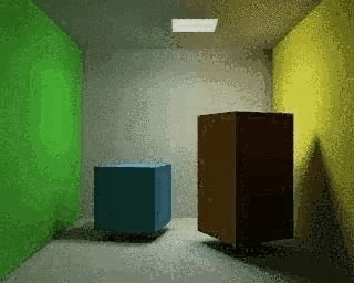
Now the Gouraud shaded faces display the energy as vertex colors. You can clearly see the 'color bleeding' in the walls, the influence of a colored object near a neutral light-grey surface. In this phase you can do some postprocess editing to reduce the number of faces or filter the colors. These are described in detail in the next section.
To leave the Radiosity mode and save the results press "Replace Meshes" and "Free Radio Data". Now we have a new Mesh Object with vertex colors. There's also a new Material added with the right proprties to render it (Press F5 or F12).
The same steps can be done with the examples "room.blend" and "radio2.blend".

[subsection]The Blender Radiosity method
During the later eighties and early nineties radiosity was a hot topic in 3D computer graphics. Many different methods were developed. The most successful solutions were based at the "progressive refinement" method with an "adaptive subdivision" scheme. (Recomended further reading: the web is stuffed with articles about radiosity, and almpost every recent book about 3D graphics covers this area. The best still is "Computer Graphics" by Foley & van Dam et al.).
To be able to get the most out of the Blender Radiosity method, it is important to understand the following principles:
Finite Element Method
Many computer graphics or simulation methods assume a simplification of reality with 'finite elements'. For a visual attractive (and even scientifically proven) solution, it is not always necessary to dive into a molecular level of detail. Instead, you can reduce your problem to a finite number of representative and well-described elements. It is a common fact that such systems quickly converge into a stable and reliable solution. The Radiosity method is a typical example of a finite element method.
Patches and Elements
In the radiosity universe, we distinguish between two types of 3D faces:
Patches. These are triangles or squares which are able to send energy. For a fast solution it is important to have as few of these patches as possible. But, because the energy is only distributed from the Patch's center, the size should be small enough to make a realistic energy distribution. (For example, when a small object is located above the Patch center, all energy the Patch sends then is obscured by this object).
Elements. These are the triangles or squares used to receive energy. Each Element is associated to a Patch. In fact, Patches are subdivided into many small Elements. When an element receives energy it absorbs part of it (depending on the Patch color) and passes the remainder to the Patch. Since the Elements are also the faces that we display, it is important to have them as small as possible, to express subtle shadow boundaries.
Progressive Refinement
This method starts with examining all available Patches. The Patch with the most 'unshot' energy is selected to shoot all its energy to the environment. The Elements in the environment recieve this energy, and add this to the 'unshot' energy of their associated Patches. Then the process starts again for the Patch NOW having the most unshot energy.
This continues for all the Patches until no energy is received anymore, or until the 'unshot' energy has converged below a certain value.
The hemicube method
The calculation of how much energy each Patch gives to an Element is done through the use of 'hemicubes'. Exactly located at the Patch's center, a hemicube consist of 5 small images of the environment. For each pixel in these images, a certain visible Element is color-coded, and the transmitted amount of energy can be calculated. Especially by the use of specialized hardware the hemicube method can be accellerated significantly. In Blender, however, hemicube calculations are done "in software".
This method is in fact a simplification and optimisation of the 'real' radiosity fomula (form factor differentiation). For that reason the resolution of the hemicube (the number of pixels of its images) is important to prevent aliasing artefacts.
Adaptive subdivision
Since the subdivision of a Mesh defines the quality of the Radiosity solution, automatic subdivision schemes have been developed to define the optimal size of Patches and Elements. Blender has two automatic subdivision methods:
Subdivide-shoot Patches. By shooting energy to the environment, and comparing the hemicube values with the actual mathematical 'form factor' value, errors can be detected that indicate a need for further subdivision of the Patch. The results are smaller Patches and a longer solving time, but a higher realism of the solution.
Subdivide-shoot Elements. By shooting energy to the environment, and detecting high energy changes (frequencies) inside a Patch, the Elements of this Patch are subdivided one exta level. The results are smaller Elements and a longer solving time and probably more aliasing, but a higher level of detail.
Display and Post Processing
Subdividing Elements in Blender is 'balanced', that means each Element differs a maximum of '1' subdivide level with its neighbours. This is important for a pleasant and correct display of the Radiosity solution with Gouraud shaded faces.
Usually after solving, the solution consists of thousands of small Elements. By filtering these and removing 'doubles', the number of Elements can be reduced significantly without destroying the quality of the Radiosity solution.
Blender stores the energy values in 'floating point' values. This makes settings for dramatic lighting situations possible, by changing the standard multiplying and gamma values.
Rendering and integration in the Blender environment
The final step can be replacing the input Meshes with the Radiosity solution (button "Replace Meshes"). At that moment the vertex colors are converted from a 'floating point' value to a 24 bits RGB value. The old Mesh Objects are deleted and replaced with one or more new Mesh Objects. You can then delete the Radiosity data with "Free Data". The new Objects get a default Material that allows immediate rendering. Two settings in a Material are important for working with vertex colors:
VColPaint. This option treats vertex colors as a replacement for the normal RGB value in the Material. You have to add Lamps in order to see the radiosity colors. In fact, you can use Blender lighting and shadowing as usual, and still have a neat radiosity 'look' in the rendering.
VertexCol. This option better should have been called "VertexLight". The vertexcolors are added to the light when rendering. Even without Lamps, you can see the result. With this option, the vertex colors are pre-multiplied by the Material RGB color. This allows fine-tuning of the amount of 'radiosity light' in the final rendering.
[subsection]The RadiosityButtons
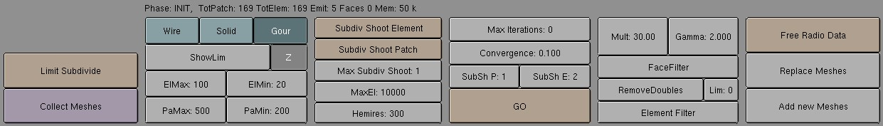
As with everything in Blender, Radiosity settings are stored in a datablock. It is attached to a Scene, and each Scene in Blender can have a different Radiosity 'block'. Use this facility to divide complex environments into Scenes with independent Radiosity solvers.
Phase 1: preparing the models
Only Meshes in Blender are allowed as input for Radiosity. It is important to realize that each face in a Mesh becomes a Patch, and thus a potential energy emittor and reflector. Typically, large Patches send and receive more energy than small ones. It is therefore important to have a well-balanced input model with Patches large enough to make a difference!
When you add extremely small faces, these will (almost) never receive enough energy to be noticed by the "progressive refinement" method, which only selects Patches with large amounts of unshot energy.
You assign Materials as usual to the input models. The RGB value of the Material defines the Patch color. The 'Emit' value of a Material defines if a Patch is loaded with energy at the start of the Radiosity simulation. The "Emit" value is multiplied with the area of a Patch to calculate the initial amount of unshot energy.
Textures in a Material are not taken account for.
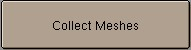
Collect Meshes
All selected and visible Meshes in the current Scene are converted to Patches. As a result some Buttons in the interface change color. Blender now has entered the Radiosity mode, and other editing functions are blocked until the button "Free Data" has been pressed. The "Phase" text prints the number of input patches. Important: check the number of "emit:" patches, if this is zero nothing interesting can happen!
Default, after the Meshes are collected, they are drawn in a pseudo lighting mode that clearly differs from the normal drawing. The 'collected' Meshes are not visible until "Free Radio Data" has been invoked.
Phase 2: subdivision limits.
Blender offers a few settings to define the minimum and maximum sizes of Patches and Elements.
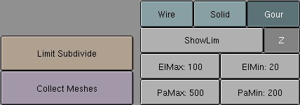
Limit Subdivide
With respect to the values "PaMax" and "PaMin", the Patches are subdivided. This subdivision is also automatically performed when a "GO" action has started.
PaMax, PaMin, ElMax, ElMin
The maximum and minimum size of a Patch or Element. These limits are used during all Radiosity phases. The unit is expressed in 0,0001 of the boundbox size of the entire environment.
ShowLim, Z
This option visualizes the Patch and Element limits. By pressing the 'Z' option, the limits are drawn rotated differently. The white lines show the Patch limits, cyan lines show the Element limits.
Wire, Solid, Gour
Three drawmode options are included which draw independent of the indicated drawmode of a 3DWindow. Gouraud display is only performed after the Radiosity process has started.
Hemires
The size of a hemicube; the color-coded images used to find the Elements that are visible from a 'shoot Patch', and thus receive energy. Hemicubes are not stored, but are recalculated each time for every Patch that shoots energy. The "Hemires" value determines the Radiosity quality and adds significantly to the solving time.
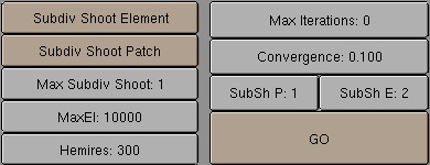
MaxEl
The maximum allowed number of Elements. Since Elements are subdivided automatically in Blender, the amount of used memory and the duration of the solving time can be controlled with this button. As a rule of thumb 20,000 elements take up 10 Mb memory.
Max Subdiv Shoot
The maximum number of shoot Patches that are evaluated for the "adaptive subdivision" (described below) . If zero, all Patches with 'Emit' value are evaluated.
Subdiv Shoot Patch
By shooting energy to the environment, errors can be detected that indicate a need for further subdivision of Patches. The subdivision is performed only once each time you call this function. The results are smaller Patches and a longer solving time, but a higher realism of the solution. This option can also be automatically performed when the "GO" action has started. Subdiv Shoot Element (But) By shooting energy to the environment, and detecting high energy changes (frequencies) inside a Patch, the Elements of this Patch are selected to be subdivided one exta level. The subdivision is performed only once each time you call this function. The results are smaller Elements and a longer solving time and probably more aliasing, but a higher level of detail. This option can also be automatically performed when the "GO" action has started.
GO
With this button you start the Radiosity simulation. The phases are:
Limit Subdivide. When Patches are too large, they are subdivided.
Subdiv Shoot Patch. The value of "SubSh P" defines the number of times the "Subdiv Shoot Patch" function is called. As a result, Patches are subdivided.
Subdiv Shoot Elem. The value of "SubSh E" defines the number of times the "Subdiv Shoot Element" function is called. As a result, Elements are subdivided.
Subdivide Elements. When Elements are still larger than the minimum size, they are sibdivided. Now, the maximum amount of memory is usually allocated.
Solve. This is the actual 'progressive refinement' method. The mousecursor displays the iteration step, the current total of Patches that shot their energy in the environment. This process continues until the unshot energy in the environment is lower than the "Convergence" or when the maximum number of iterations has been reached.
Convert to faces. The elements are converted to triangles or squares with 'anchored' edges, to make sure a pleasant not-discontinue Gouraud display is possible.
SubSh P
The number of times the environment is tested to detect Patches that need subdivision. (See option: "Subdiv Shoot Patch").
SubSh E
The number of times the environment is tested to detect Elements that need subdivision. (See option: "Subdiv Shoot Element").
Convergence
When the amount of unshot energy in an environment is lower than this value, the Radiosity solving stops. The initial unshot energy in an environment is multiplied by the area of the Patches. During each iteration, some of the energy is absorped, or disappears when the environment is not a closed volume. In Blender's standard coordinate system a typical emittor (as in the example files) has a relative small area. The convergence value in is divided by a factor of 1000 before testing for that reason .
Max iterations
When this button has a non-zero value, Radiosity solving stops after the indicated iteration step.
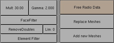
Element Filter
This option filters Elements to remove aliasing artefacts, to smooth shadow boundaries, or to force equalized colors for the "RemoveDoubles" option.
RemoveDoubles
When two neighbouring Elements have a displayed color that differs less than "Lim", the Elements are joined.
Lim
This value is used by the previous button. The unit is expressed in a standard 8 bits resolution; a color range from 0 - 255.
FaceFilter
Elements are converted to faces for display. A "FaceFilter" forces an extra smoothing in the displayed result, without changing the Element values themselves.
Mult, Gamma
The colorspace of the Radiosity solution is far more detailed than can be expressed with simple 24 bit RGB values. When Elements are converted to faces, their energy values are converted to an RGB color using the "Mult" and "Gamma" values. With the "Mult" value you can multiply the energy value, with "Gamma" you can change the contrast of the energy values.